
using GLMakie
using Distributions

function partA(τ::Float64, σ::Float64)
    # define the length of subintervals
    Δt = 1e-4
    ts = 0.0:Δt:5.0
    # number of samples
    N = 5
    # Weiner processs
    W = Normal(0, sqrt(Δt))
    # initialize mesh
    X = Matrix{Float64}(undef, length(ts), N)
    Y = Matrix{Float64}(undef, length(ts), N)

    # apply initial conditions
    for i in 1:N
        X[1, i] = rand()
        Y[1, i] = rand()
    end
    # propagate the process
    for i in 1:N
        for j in 2:length(ts)
            ΔW = rand(W)
            X[j, i] = X[j-1, i] - (X[j-1, i]^3)*Δt -τ*Y[j-1, i]*Δt + σ*ΔW
            Y[j, i] = Y[j-1, i] - τ*Y[j-1, i]*Δt + σ*ΔW
        end
    end
    # make the figure
    fig = Figure()
    ax = Axis(
        fig[1, 1],
        title = "σ = $σ τ = $τ",
        xlabel = "t",
        ylabel = L"$X_{n+1}$"
    )
    # set y axis limits
    ylims!(ax, -1.0, 1.0)

    # Plot the samples
    for i in 1:N
        lines!(ax, ts, X[:, i])
    end
    return fig
end
save("parta01.png", partA(0.01, 0.1))
save("parta1.png", partA(1.0, 0.1))
save("parta10.png", partA(10.0, 0.1))Homework 4
Question 1
Consider the system of SDEs
\[\begin{cases}dX(t;\omega) &= -X(t;\omega)^3dt + dY(t;\omega) \\dY(t;\omega) &= -\tau Y(t;\omega)dt + \sigma dW(t;\omega)\end{cases} \tag{1}\]
where \(\sigma, \tau \leq 0\) are given parameters and \(W(t;\omega)\) is a Wiener process. The initial condition \((X(0;\omega), Y(0;\omega))\) has i.i.d. components both of which are uniformly distributed in \([0, 1]\), i.e., \(X(0;\omega)\) and \(Y(0;\omega)\) are independent random variables with uniform PDF in \([0,1]\).
Part A
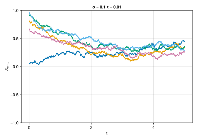
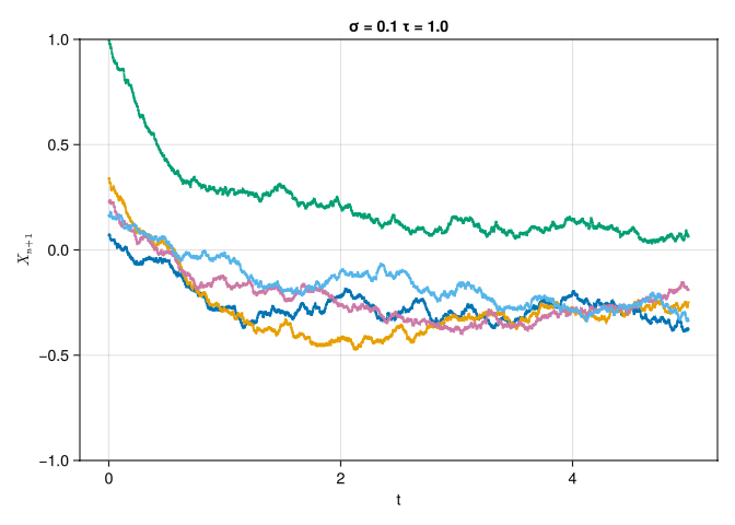
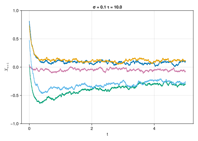
Plot a few sample paths of \(X(t;\omega)\) for \(\sigma = 0.1\) and \(\tau = \{0.01, 1, 10\}\).
Solution
We convert Equation 1 into a numerical simulation by first converting the SDE into a discrete time form via the Euler-Maruyama discretization.
We descritize a grid within the interval [0, T] into N equal parts, where \(\Delta t = \frac{T}{N}\)
Let us recursively define \(Y_n\) for \(0 \leq n \leq N-1\)
\[\begin{align} Y_{n+1} = Y_n -\tau Y_n \Delta t + \sigma \Delta W \end{align}\]
and \(X_n\)
\[\begin{align} X_{n+1} = X_n - X_n^3 \Delta t + \Delta Y_n \end{align}\]
where \(\Delta Y_n = Y_{n+1} - Y_n = -\tau Y_n \Delta t + \sigma \Delta W_n\)
where \(\Delta W_n\) are i.i.d Gaussian random variables with zero mean and variance \(\Delta t\).
Part B
Do you expect the system Equation 1 to have a statistically stationary state? Justify your answer.
Solution
From part A, we can see that as we increase \(\tau\), the system rapidly converges to a statistically steady-state process. We can prove this by the Kernel Density Estimation for 1000 sample paths for varying \(\tau\) and comparing the estimated PDF for later times.
The solution approaches a statistically steady state as \(t\rightarrow \infty\) and approaches the statisically steady state at the rate \(\tau\). It seems though that the pdf for varying \(\tau\) may not be the same, as \(\tau = 10.0\) seems to have a bimodal distribution for later times.
using KernelDensity

function simulateB(τ::Float64)
    σ = 0.1
    # define the length of subintervals
    Δt = 1e-4
    ts = 0.0:Δt:20.0
    # number of samples
    N = 1000
    # Weiner processs
    W = Normal(0, sqrt(Δt))
    # initialize mesh
    X = Matrix{Float64}(undef, length(ts), N)
    Y = Matrix{Float64}(undef, length(ts), N)

    # apply initial conditions
    for i in 1:N
        X[1, i] = rand()
        Y[1, i] = rand()
    end
    # propagate the process
    for i in 1:N
        for j in 2:length(ts)
            ΔW = rand(W)
            X[j, i] = X[j-1, i] - (X[j-1, i]^3)*Δt -τ*Y[j-1, i]*Δt + σ*ΔW
            Y[j, i] = Y[j-1, i] - τ*Y[j-1, i]*Δt + σ*ΔW
        end
    end
    return X, Y, length(ts)
end

function partB()
    X1, Y1, ts = simulateB(0.01)
    X2, Y2, _ = simulateB(1.0)
    X3, Y3, _ = simulateB(10.0)

    fig = Figure()
    ax = Axis(
        fig[1, 1]
    )
    ylims!(ax, 0.0, 3.0)
    xlims!(ax, -2.0, 2.0)

    d1 = kde(X1[1, :])
    d2 = kde(X2[1, :])
    d3 = kde(X3[1, :])
    kde_data1 = Observable((d1.x, d1.density))
    kde_data2 = Observable((d2.x, d2.density))
    kde_data3 = Observable((d3.x, d3.density))

    kde_line1 = lines!(ax, [0.0], [0.0], color = :red, label = "τ = 0.01")
    kde_line2 = lines!(ax, [0.0], [0.0], color = :blue, label = "τ = 1.0")
    kde_line3 = lines!(ax, [0.0], [0.0], color = :green, label = "τ = 10.0")

    kde_plot1 = lift(kde_data1) do (x, density)
        kde_line1[1] = x
        kde_line1[2] = density
    end
    kde_plot2 = lift(kde_data2) do (x, density)
        kde_line2[1] = x
        kde_line2[2] = density
    end
    kde_plot3 = lift(kde_data3) do (x, density)
        kde_line3[1] = x
        kde_line3[2] = density
    end

    Legend(fig[1, 2], ax)
    record(fig, "partb.mp4", 2:400:ts; framerate = 30) do k
        d1 = kde(X1[k, :])
        d2 = kde(X2[k, :])
        d3 = kde(X3[k, :])
        kde_data1[] = (d1.x, d1.density)
        kde_data2[] = (d2.x, d2.density)
        kde_data3[] = (d3.x, d3.density)
    end
    return fig
end
partB()
Part C
Write the Fokker-Planck equation for the joint PDF of \(X(t;\omega)\) and \(Y(t;\omega)\).
Solution
Let us write Equation 1 in state-space form
\[\begin{align} dX &= -X^3 dt - \tau Y dt + \sigma dW \\ dY &= -\tau Y dt + \sigma dW \end{align}\]
The vector \(\mathbf{G}(\mathbf{X}, t)\) can be written as
\[\begin{align} \mathbf{G}(\mathbf{X}, t) &= \left[ \begin{matrix} -X^3 - \tau Y \\ -\tau Y \end{matrix}\right] \end{align}\]
The matrix \(\mathbf{S}\) can be written as
\[\begin{align} \mathbf{S} = \left[ \begin{matrix} \sigma \\ \sigma \end{matrix}\right] \end{align}\]
We can thus write the Fokker-Planck equation according equation 59 in course notes 4 as follows:
\[\begin{align} \frac{\partial p(\mathbf{x}, t)}{\partial t} &= -\sum_{k=1}^{2} \frac{\partial}{\partial x_k} \left(G_k(\mathbf{x}, t) p(\mathbf{x})\right) + \frac{1}{2} \sum_{i, k = 1}^2 \frac{\partial^2}{\partial x_i \partial x_k}\left(\sum_{j=1}^2 S_{ij}(\mathbf{x}, t)S_{kj}(\mathbf{x}, t) p(\mathbf{x}, t) \right) \\ \frac{\partial p}{\partial t} &= -\left(\frac{\partial}{\partial x} \left((-x^3 -\tau y)p\right) + \frac{\partial}{\partial y}\left(-\tau yp\right)\right) + \frac{\sigma^2}{2}\left(\frac{\partial^2p}{\partial x^2} + \frac{\partial^2 p}{\partial y^2}\right) \\ &= \frac{\partial}{\partial x}(x^3 p) + \tau p + \tau y\left(\frac{\partial p}{\partial x} + \frac{\partial p}{\partial y}\right) + \frac{\sigma^2}{2}\left(\frac{\partial^2p}{\partial x^2} + \frac{\partial^2 p}{\partial y^2}\right) \end{align}\]
The Fokker-Planck equation is thus
\[\frac{\partial p(x, y, t)}{\partial t} = \frac{\partial}{\partial x}(x^3 p(x, y, t)) + \tau p(x, y, t) + \tau y\left(\frac{\partial p(x, y, t)}{\partial x} + \frac{\partial p(x, y, t)}{\partial y}\right) + \frac{\sigma^2}{2}\left(\frac{\partial^2p(x, y, t)}{\partial x^2} + \frac{\partial^2 p(x, y, t)}{\partial y^2}\right) \tag{2}\]
where \(p(x, y, t)\) is the joint PDF of \(X\) and \(Y\).
Part D
Write the reduced-order equation for the joint PDF of \(X(t;\omega)\) in terms of the conditional expectation \(\mathbb{E}\{Y(t;\omega)|X(t;\omega)\}\).
Solution
To obtain the reduced-order equation, let us integrate Equation 2 with respect to \(y\) and use the definition of conditional PDF.
\[\begin{align} \frac{\partial}{\partial t}\int_{-\infty}^{\infty}pdy &= \int_{-\infty}^{\infty}\left(\frac{\partial}{\partial x} \left((x^3 +\tau y)p\right) + \frac{\partial}{\partial y}\left(\tau yp\right) + \frac{\sigma^2}{2}\left(\frac{\partial^2p}{\partial x^2} + \frac{\partial^2 p}{\partial y^2}\right)\right) dy\\ \frac{\partial p(x,t)}{\partial t} &= \frac{\partial}{\partial x} \int_{-\infty}^{\infty}(x^3 + \tau y)p dy + \int_{-\infty}^{\infty} \frac{\partial}{\partial y}(\tau yp)dy + \frac{\sigma^2}{2}\left(\frac{\partial^2}{\partial x^2}\int_{-\infty}^{\infty}p dy + \cancelto{0}{\int_{-\infty}^{\infty}\frac{\partial^2 p}{\partial y^2}dy}\right) \\ &= \frac{\partial}{\partial x}\left(x^3p(x, t) + \tau p(x, t)\mathbb{E}\{Y | X\}\right) + \cancelto{0}{\tau y p_{\bigg{|}_{-\infty}^{\infty}}} + \frac{\sigma^2}{2}\frac{\partial^2 p(x, t)}{\partial x^2}\\ \end{align}\]
Thus, the reduced order equation for the joint PDF can be written as,
\[\frac{\partial p(x, t)}{\partial t} = \frac{\partial}{\partial x}(x^3 p(x, t)) + \tau \frac{\partial}{\partial x}\left(p(x, t)\mathbb{E}\{y|x\}\right) + \frac{\sigma^2}{2} \frac{\partial^2 p(x, t)}{\partial x^2} \tag{3}\]
Part E
Set \(\sigma = 0\). Compute the conditional expectation \(\mathbb{E}\{Y(t;\omega) | X(t;\omega)\}\) explicity as a function of \(t\) and substitute it in the reduced order equation you obtained in part d (with \(\sigma = 0\)) to obtain an exact (and closed) equation for the PDF of \(X(t;\omega)\).
Solution
Recall the orginal SDE Equation 1 where
\[\begin{align} dY = -\tau Y dt + \sigma dW \end{align}\]
setting \(\sigma = 0\) we have the following ODE:
\[\begin{align} \begin{cases} \frac{dY}{dt} = -\tau Y \\ Y(0) \sim \text{Uniform}(0, 1) \end{cases} \end{align}\]
solving for \(Y(t)\) we have:
\[\begin{align} Y(t) = Y(0)e^{-\tau t} \end{align}\]
where \(Y(0)\) can be expressed as the expectation of a uniform random variable in [0, 1], which we know is \(\frac{1}{2}\)
therefore the conditional expectation \[\mathbb{E}\{Y|X\} = \mathbb{E}\{Y\} = \frac{1}{2}e^{-\tau t}\]
we can write a closed equation for the reduced order equation as follows:
\[\frac{\partial p(x, t)}{\partial t} = \frac{\partial }{\partial x}(x^3p(x, t)) + \tau \frac{\partial }{\partial x}(p(x, t)\frac{1}{2}e^{-\tau t}) \tag{4}\]
Part F
Write the PDF equation you obtained in part e as an evolution equation for the cumulative distribution function (CDF) of \(X(t;\omega)\).
Solution
Recall the definition of the cumulative distribution function:
\[\begin{align} F(x, y, t) = \int_{-\infty}^{x}p(y, t)dy \end{align}\]
if we take the derivative on both sides with respect to \(x\) we have
\[\begin{align} p(x, t) = \frac{\partial F(x, t)}{\partial x} \end{align}\]
plugging this into Equation 4 we have
\[\begin{align} \frac{\partial }{\partial t}\left(\frac{\partial F}{\partial x}\right) = \frac{\partial }{\partial x}\left(x^3\frac{\partial F}{\partial x}\right) + \tau \frac{\partial }{\partial x}\left(\frac{\partial F}{\partial x}\frac{1}{2}e^{-\tau t}\right) \end{align}\]
taking the integral of both sides:
\[\begin{align} \int_{-\infty}^{x}\frac{\partial^2 F}{\partial t\partial x'}dx' &= \int_{-\infty}^{x}\left(\frac{\partial }{\partial x'}\left(x'^3\frac{\partial F}{\partial x'}\right) + \frac{\tau}{2} \frac{\partial }{\partial x'}\left(\frac{\partial F}{\partial x'}e^{-\tau t}\right)\right)dx' \\ \frac{\partial F(x, t)}{\partial t} &= x'^3 \frac{\partial F}{\partial x'}\bigg|_{-\infty}^{x} + \frac{\tau}{2} \frac{\partial F}{\partial x'}e^{-\tau t}\bigg|_{-\infty}^{x} \\ \end{align}\]
thus we are left with the evolution equation for \(F(x, t)\)
\[\frac{\partial F(x, t)}{\partial t} = x^3 \frac{\partial F(x, t)}{\partial x} + \frac{\tau}{2}e^{-\tau t}\frac{\partial F(x, t)}{\partial x}\]