Homework 5

Author

Affiliation

Kevin Silberberg

University of California Santa Cruz

Question 1

Consider a random variable \(\xi\) with PDF

\[p_{\xi}(x) = \begin{cases} \frac{e^{-x}}{e - e^{-1}} & x \in [-1, 1] \\ 0 & \text{otherwise} \end{cases} \tag{1}\]

Part A

Use the Stieltjes algorithm to compute the sixth-order generalized polynomial choas basis \[\{P_0(x), P_1(x), ..., P_6(x)\}\] for \(\xi\), i.e. a set of polynomials up to degree 6 that are orthogonal relative to the PDF \(\xi\) given in Equation 1.

Solution

We know that since the distribution function Equation 1 is compactly supported, that the solution to the moment problem is unique and exists.

Let \(c = \frac{1}{e-e^{-1}}\) the constant in \(p_{\xi}(x)\)

Following the Stieltjes algorithm, let us compute the first orthogonal polynomial and then we will write a code that computes the first six orthogonal polynomials where \[\begin{align} \mu(x) = ce^{-x} \end{align}\]

is out weight function.

Let \(n = 0 \quad \pi_0 = 1 \quad \pi_{-1} = 0\)

\[\begin{align} \alpha_0 &= \frac{\langle x , 1 \rangle}{\langle 1, 1 \rangle} \\ &= \frac{c \int_{-1}^{1}x e^{-x}dx}{c \int_{-1}^{1}e^{-x}dx} \\ &= \frac{\left[{-x e^{-x}}_{\bigg{\vert}_{-1}^{1}} - \int_{-1}^{1}-e^{-x}dx\right]}{\left[{-e^{-x}}_{\bigg{\vert}_{-1}^{1}}\right] } \\ &= \frac{-e^{-1} - e - e^{-1} + e}{-e^{-1} + e} \\ &= -\frac{2}{e^2 - 1} \approx -0.31304 \end{align}\]

Using \(\alpha_0\) let us find the first polynomial \(\pi_1\) using the following formula

\[\begin{align} \pi_{n+1}(x) = (x - \alpha_n)\pi_n(x) - \beta_n \pi_{n-1}(x) \end{align}\]

\[\begin{align} \pi_1(x) &= (x - \alpha_0)\pi_0 - \beta_0 \pi_{-1} \\ &= x + \frac{2}{e^2 - 1} \end{align}\]

Let us now write a code that produces any arbitray number of orthogonal polynomials with respect to the weight function.

using GLMakie
using QuadGK
using StaticArrays
using Statistics

# weight function
μ(x) = exp(-x) * ^((exp(1.0) - ^(exp(1.0), -1.0)), -1.0)

# define an integral using gauss-kronrod quadrature rule
integ(x::Function, sup::SVector{2}) = quadgk(x, sup[1], sup[2]; atol=1e-8, rtol=1e-8)[1]

# the support of the weight function
sup = SVector{2}(-1.0, 1.0)

# cumulative trapazoidal rule
function cumsumtrap(f::Function, x)
    y = f.(x)
    N = length(x)
    x1 = @view x[1:N-1]
    x2 = @view x[2:N]
    y1 = @view y[1:N-1]
    y2 = @view y[2:N]
    integral = cumsum(((x2.-x1).*(y1.+y2))./2.0)
    integral ./= integral[end]
    return [0; integral]
end

# CDF inverse sampler
function sampleInverseCDF(x::Float64, points::Matrix{Float64})
    idx = findfirst(points[:, 1] .> x)
    if idx === nothing
        p1 = points[end-1, :]
        p2 = points[end, :]
    elseif idx == 1
        p1 = points[1, :]
        p2 = points[2, :]
    else
        p1 = points[idx-1, :]
        p2 = points[idx, :]
    end
    liy(x, p1, p2)
end

# Linear Interpolator
function liy(x::Float64, p1::Vector{Float64}, p2::Vector{Float64})
    x1, y1 = p1
    x2, y2 = p2
    if isapprox(x1, x2, atol = 1e-12)
        return (y1 + y2) / 2.0
    end
    return y1 + (x - x1)*(y2 - y1)/(x2 - x1)
end

# stieltjes algorithm
function stieltjes(μ::Function, N::Int64, sup::SVector{2})
    # μ: weight function defining the inner product
    # N: number of orthogonal polynomials to compute
    # sup: support (integration bounds) of the weight function

    M = N + 2  # Extend size to accommodate buffer
    n = 2      # Starting index for the recursion

    # Initialize orthogonal polynomials (πn) as functions
    π = Vector{Function}(undef, M)
    π[n-1] = x -> 0.0 * x^0.0  # π₀(x) = 0
    π[n] = x -> 1.0 * x^0.0    # π₁(x) = 1

    # Initialize coefficient vectors αn and βn
    α = Vector{Float64}(undef, M)
    β = Vector{Float64}(undef, M)
    β[n-1] = 0.0  # β₀ = 0
    β[n] = 0.0    # β₁ = 0

    # Compute the first α coefficient (α₂)
    # α₂ = ⟨xπ₁, π₁⟩ / ⟨π₁, π₁⟩
    α[n] = integ(x -> x * π[n](x) * π[n](x) * μ(x), sup) / integ(x -> π[n](x) * π[n](x) * μ(x), sup)

    # Compute the next orthogonal polynomial π₂
    # π₂(x) = (x - α₁)π₁(x) - β₁π₀(x)
    π[n+1] = x -> (x - α[n]) * π[n](x) - β[n] * π[n-1](x)

    for n in 3:M-1
        α[n] = integ(x -> x * π[n](x) * π[n](x) * μ(x), sup) / integ(x -> π[n](x) * π[n](x) * μ(x), sup)
        β[n] = integ(x -> π[n](x) * π[n](x) * μ(x), sup) / integ(x -> π[n-1](x) * π[n-1](x) * μ(x), sup)
        π[n+1] = π[n+1] = x -> (x - α[n]) * π[n](x) - β[n] * π[n-1](x)
    end
    return π
end
π = stieltjes(μ, 6, sup)

8-element Vector{Function}:
 #1 (generic function with 1 method)
 #2 (generic function with 1 method)
 #5 (generic function with 1 method)
 #10 (generic function with 1 method)
 #10 (generic function with 1 method)
 #10 (generic function with 1 method)
 #10 (generic function with 1 method)
 #10 (generic function with 1 method)

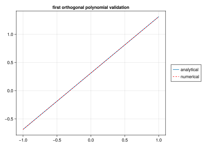
Let us define a function that plots the first polynomial \(\pi_1(x)\) over the numerical result as a validation.

function validatepione(π::Vector{Function})
    π_1(x) = x + (2 / (exp(1)^2 - 1))
    xs = LinRange(-1, 1, 1000)
    fig = Figure()
    ax = Axis(fig[1, 1], title = "first orthogonal polynomial validation")
    lines!(ax, xs, π_1.(xs), label = "analytical")
    lines!(ax, xs, π[3].(xs), label = "numerical", linestyle = :dash, color = :red)
    Legend(fig[1, 2], ax)
    save("validationpione.png", fig)
end
validatepione(π);

Validation of the stieltjes algorthim: Plot of numerical over analytical solution of the first orthogonal polynomial

Part B

Veriy that the polynomial basis you obtained in part a is orthogonal, i.e., that the matrix

\[\mathbb{E}\{P_k(\xi)P_j(\xi)\} = \int_{-1}^{1} P_k(x)P_j(x)dx \tag{2}\]

is diagonal.

Solution

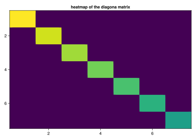
Let us write a code that computes the Matrix and then plot the matrix using a heatmap to check if it diagonal.

function isdiagonal(π::Vector{Function}, sup::SVector{2})
    A = Matrix{Float64}(undef, 7, 7)
    for idx in CartesianIndices(A)
        (k, j) = idx.I
        ele = integ(x-> π[k+1](x) * π[j+1](x) * μ(x), sup)
        A[k, j] = ele < 1e-12 ? 1e-8 : ele
    end
    fig = Figure()
    ax = Axis(fig[1, 1], title = "heatmap of the diagona matrix")
    heatmap!(ax, log10.(A))
    ax.yreversed=true
    save("heatmapdiagonal.png", fig)
end
isdiagonal(π, sup)

Heatmap showing that the matrix of innerproducts with respect to the weight function of all polynomials generated is diagonal.

Clearly we can see that the matrix is diagonal and thus the polynomial functions are orthogonal with respect to the weight function.

Part C

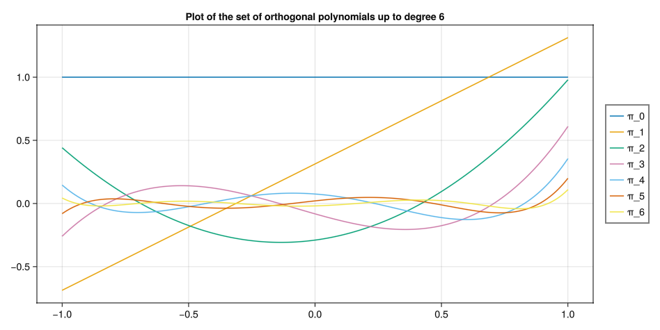
Plot \(P_k(x)\) for \(k = 0, ..., 6\)

Solution

Let us define a code that plots all polynomials \(P_k(x)\) for \(k = 0, ..., 6\)

function plotpolynomials(π::Vector{Function})
    M = size(π)[1]
    fig = Figure();display(fig)
    ax = Axis(fig[1, 1], title = "Plot of the set of orthogonal polynomials up to degree 6")
    xs = LinRange(-1.0, 1.0, 1000)
    for n in 1:M-1
        lines!(ax, xs, π[n+1].(xs), label="π_$(n-1)")
    end
    Legend(fig[1, 2], ax)
    save("plotpolynomials.png", fig)
end
plotpolynomials(π)

Plot of polynomials within the support [-1, 1]

Question 2

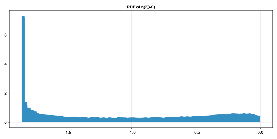
Consider the following nonlinear fuction of the random variable \(\xi(\omega)\) with PDF defined in Equation 1

\[\eta(\omega) = \frac{\xi(\omega) -1}{2 + 1\sin{(2\xi(\omega))}} \tag{3}\]

Part A

Compute the PDF of \(\eta\) using the relative frequency approach. To this end, sample 50,000 realizations of \(\xi\) using the inverse CDF approach applied to Equation 1, and use such samples to compute samples of \(\eta(\omega)\).

Solution

The following code samples from Equation 1 50,000 times using the inverse sampling method previously applied in Homework 1 and 2, then applies the transformation Equation 3, and finally plots the histogram with 80 bins, normalized so that the PDF integrates to one over the support.

η(ξ) = (ξ - 1) / (2 + sin(2*ξ))
function question2a()
    r = LinRange(-1, 1, 1000)
    fig = Figure();display(fig)
    ax = Axis(fig[1, 1],
        title = "PDF of η(ξ(ω))")
    ys = cumsumtrap(μ, r)
    samples = Vector{Float64}(undef, 50000)
    for i in eachindex(samples)
        samples[i] = η(sampleInverseCDF(rand(), hcat(ys, r)))
    end
    hist!(ax, samples, bins = 80, normalization = :pdf)
    save("question2a.png", fig)
    samples
end
samples = question2a();

PDF of \(\eta(\xi(\omega))\) by sampling 50,000 times via inverse CDF approach and applying the transformation Equation 3

Part B

Show numerically that the gPC expansion ¹

\[\eta_M(\omega) = \sum_{k=0}^{M}a_k P_k(\xi(\omega)), \quad a_k = \frac{\mathbb{E}\{\eta(\xi(\omega))P_k(\xi(\omega))\}}{\mathbb{E}\{P_k^2(\xi(\omega))\}} \tag{5}\]

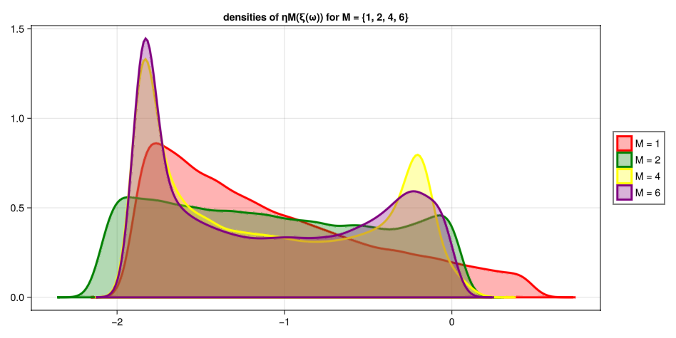
converges to \(\eta(\omega)\) in distribution as \(M\) increases. To this end, plot the PDF of the random variables \(\eta_M(\xi(\omega))\) for \(M = 1, 2, 4, 6\) using method of relative frequencies and compare such PDF’s with the PDF of \(\eta\) you computed in part a.

Solution

function question2b(πn::Vector{Function})
    a = Vector{Float64}(undef, 7)
    colors = Symbol[:red, :green, :blue, :yellow, :orange, :purple]
    # calculate coefficients
    for k in eachindex(a)
        a[k] = integ(x -> η(x) * πn[k+1](x) * μ(x), sup) / integ(x -> πn[k+1](x) * πn[k+1](x) * μ(x), sup)
    end

    fig = Figure();display(fig)
    ax = Axis(fig[1, 1], title="densities of ηM(ξ(ω)) for M = {1, 2, 4, 6}")
    r = LinRange(-1, 1, 1000)
    ys = hcat(cumsumtrap(μ, r), r)
    for M in SVector{4}(1, 2, 4, 6)
        ηM_samples = Vector{Float64}(undef, 50000)
        for l in eachindex(ηM_samples)
            η_sum = 0.0
            ξ = sampleInverseCDF(rand(), ys)
            for k in 1:M+1
                η_sum+=a[k]*πn[k+1](ξ)
            end
            ηM_samples[l] = η_sum
        end
        density!(ax, ηM_samples, color = (colors[M], 0.3), label = "M = $M", strokecolor = colors[M], strokewidth = 3, strokearound = true)
    end
    Legend(fig[1, 2], ax)
    save("question2b.png", fig)
end
question2b(π);

The PDF ploted using Kernel Density Estimation for values M = {1, 2, 4, 6}

As we can see, the PDF of the random variable \(\eta_M(\omega)\) converges to the PDF of \(\eta(\omega)\) as M increases.

Part C

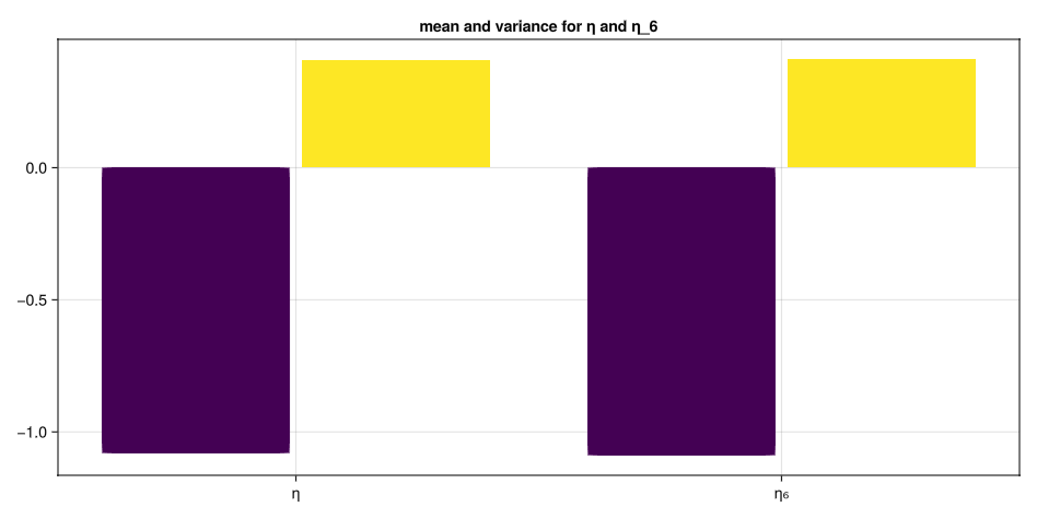
Compute the mean and variance of \(\eta_6\) and compare it with the mean and variance of \(\eta\). Note that such means and variances can be computed in multiple ways, e.g., by using MC, or by approximating the integral defining the moments of the random variable \(\eta\) using quadrature, e.g., via the trapezoidal rule applied to the integral

\[\mathbb{E}\{\eta^k\} = \int_{-1}^{1} \left(\frac{x-1}{2+\sin(2x)}\right)^k p_{\xi}(x)dx \tag{6}\]

Solution

Let us find the mean and variance of \(\eta\) and \(\eta_6\) by generating 1000 samples of size 1000 and taking the average of the mean and variance for each sample.

function question2c()
    πn = stieltjes(μ, 6, sup)
    r = LinRange(-1, 1, 1000)
    ys = hcat(cumsumtrap(μ, r), r)
    η_samples = Vector{Float64}(undef, 50000)
    for i in eachindex(η_samples)
        η_samples[i] = η(sampleInverseCDF(rand(), ys))
    end
    a = Vector{Float64}(undef, 7)
    for k in eachindex(a)
        a[k] = integ(x -> η(x) * πn[k+1](x) * μ(x), sup) / integ(x -> πn[k+1](x) * πn[k+1](x) * μ(x), sup)
    end
    η6_samples = Vector{Float64}(undef, 50000)
    for l in eachindex(η6_samples)
        η_sum = 0.0
        ξ = sampleInverseCDF(rand(), ys)
        for k in eachindex(a)
            η_sum+=a[k]*πn[k+1](ξ)
        end
        η6_samples[l] = η_sum
    end

    means = Vector{Float64}(undef, 1000)
    variances = Vector{Float64}(undef, 1000)
    for i in eachindex(means)
        sample = rand(η_samples, 1000)
        means[i] = mean(sample)
        variances[i] = var(sample)
    end
    η_mean = mean(means)
    η_var = mean(variances)

    means = Vector{Float64}(undef, 1000)
    variances = Vector{Float64}(undef, 1000)
    for i in eachindex(means)
        sample = rand(η6_samples, 1000)
        means[i] = mean(sample)
        variances[i] = var(sample)
    end
    η6_mean = mean(means)
    η6_var = mean(variances)
    fig = Figure();display(fig)
    ax = Axis(fig[1, 1],
        xticks = (1:2, ["η", "η₆"]),
    title = "mean and variance for η and η_6")
    barplot!(ax, [1, 1, 2, 2], [η_mean, η_var, η6_mean, η6_var],
        dodge = [1, 2, 1, 2],
        color = [1, 2, 1, 2])
    save("question2c.png", fig)
end
question2c();

Barplot of the bootstrap mean and variance from MC for \(\eta\) and \(\eta_6\)

From the plot we can see the the sample mean and variance for both are almost identical.

Question 3

Compute the solution of the following random initial value problem

\[\begin{cases} \frac{dx}{dt} &= -\xi(\omega)x + \cos(4t) \\ x(0) &= 1 \end{cases} \tag{7}\]

using the stocastic Galerkin method with the gPC basis you obtained in question 1. In particular, use the following gPC expansion of degree 6 for the solution of Equation 7.

\[x(t;\omega) = \sum_{k=0}^6 \hat{x}_k(t)P_k(\xi(\omega)) \tag{8}\]

where the gPC modes \(\hat{x}_k(t)\) are to be determined from Equation 7.

Part A

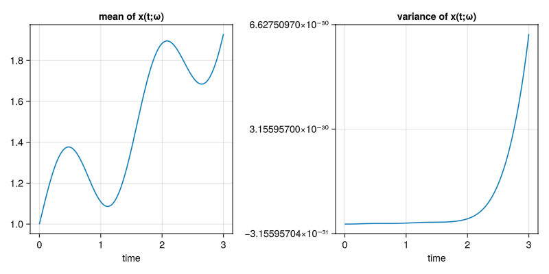
Compute the mean and the variance of Equation 8 of \(t \in [0, 3]\).

Solution

Let us find the solution of the random initial value problem by using the stocastic Galerkin method and finding the gPC modes by plugging in Equation 8 into Equation 7.

\[\begin{align} \sum_{k=0}^{6}\frac{\partial \hat{x}_k}{\partial t}P_k &= -\xi \sum_{k=0}^{6}\hat{x}_k P_k + cos(4t) \\ \frac{\partial \hat{x}_j}{\partial t}\mathbb{E}\{P_j^2\} &= -\sum_{k=0}^{6}\hat{x}_k \mathbb{E}\{\xi P_k P_j\} + \cos(4t) \mathbb{E}\{P_j\} \\ \frac{\partial \hat{x}_j}{\partial t} &= -\frac{1}{\mathbb{E}\{P_j^2\}}\sum_{k=0}^{6}\hat{x}_k \mathbb{E}\{\xi P_k P_j\} + \frac{\cos(4t) \mathbb{E}\{P_j\}}{\mathbb{E}\{P_j^2\}} \\ \end{align}\]

Recall from Question 1, Part A where we calculated the \(P_1(\xi)\)

\[\begin{align} P_1(\xi) &= \xi + \frac{2}{e^2 + 1} \\ \xi &= P_1(\xi) - \frac{2}{e^2 + 1} \end{align}\]

Plugging \(\xi\) back into the ODE we have:

\[\begin{align} \frac{\partial \hat{x}_j}{\partial t} &= -\frac{1}{\mathbb{E}\{P_j^2\}}\sum_{k=0}^{6}\hat{x}_k \mathbb{E}\{ \left(P_1(\xi) - \frac{2}{e^2 + 1}\right) P_k P_j\} + \frac{\cos(4t) \mathbb{E}\{P_j\}}{\mathbb{E}\{P_j^2\}} \\ \frac{\partial \hat{x}_j}{\partial t} &= -\frac{1}{ \mathbb{E}\{P_j^2\}} \sum_{k=0}^{6}\hat{x}_k \mathbb{E}\{P_1 P_k P_j\} + \frac{2\hat{x}}{e^2 + 1} + \frac{\cos(4t) \mathbb{E}\{P_j\}}{ \mathbb{E}\{P_j^2\}} \end{align}\]

where the initial conditions are:

\[\begin{align} x(0;\omega) &= 1 \\ x(j;\omega) &= 0 \quad \text{for } j = 1, ..., 6 \end{align}\]

In the following code we precompute the expectations required for defining the first order system of equations, solve the IVP using Tsitouras 5/4 Runge-Kutta method, calculate the variance by the following:

\[\begin{align} var(x(t;\omega)) = \sum_{k=1}^{6}\hat{x}_k^2(t) \mathbb{E}\{P_k^2\} \end{align}\]

and plot the mean and variance on two seperate graphs in the temporal domain [0, 3]

using DifferentialEquations
function question3a()
    # get polynomials
    πn = stieltjes(μ, 6, sup)

    # simulation initial and final time
    t0, tf = SVector{2}(0.0, 3.0)

    # initial conditions
    u0 = SVector{7}(1, 0, 0, 0, 0, 0, 0)

    # highest polynomial order
    M = size(πn)[1] - 1

    # precompute E{Pj}
    Epj1 = Vector{Float64}(undef, M)
    for k in eachindex(Epj1)
        Epj1[k] = integ(x -> πn[k+1](x) * μ(x), sup)
    end

    # precompute E{Pj^2}
    Epj2 = Vector{Float64}(undef, M)
    for j in eachindex(Epj2)
            Epj2[j] = integ(x -> πn[j+1](x) * πn[j+1](x) * μ(x), sup)
    end

    # precompute E{P₁PkPj}
    Ep1pjpk = Matrix{Float64}(undef, M, M)
    for idx in CartesianIndices(Ep1pjpk)
        (j, k) = idx.I
        Ep1pjpk[j, k] = integ(x -> πn[2](x) * πn[j+1](x) * πn[k](x) * μ(x), sup)
    end

    # precompute the constant multiplying xhatj
    β = (2.0 / (exp(1.0)^2 + 1.0))

    # define the system of odes
    function ode(u, p, t)
        return SVector{M}(
            ((-sum(u[k] * Ep1pjpk[j, k] for k in 1:M))/Epj2[j]) + β*u[j] + (cos(4*t)*Epj1[j]/Epj2[j]) for j in 1:M
        )
    end

    # solve the ode problem using Tsitouras 5/4 Runge-Kutta method
    prob = ODEProblem(ode, u0, (t0, tf))
    sol = solve(prob, Tsit5(), saveat=0.01, abstol=1e-8, reltol=1e-8)
    # find the variance
    var = sum([(sol[k, :].^2) .* Epj2[k] for k in 2:M], dims=1)[1]

    # plot the mean and variance
    fig = Figure(size = (800, 400));display(fig)
    ax1 = Axis(fig[1, 1], title = "mean of x(t;ω)",
        xlabel = "time")
    ax2 = Axis(fig[1, 2], title = "variance of x(t;ω)",
        xlabel = "time")
    lines!(ax1, sol.t, sol[1, :])
    lines!(ax2, sol.t, var)
    save("question3a.png", fig)
    return sol
end
question3a();

┌ Warning: No strict ticks found
└ @ PlotUtils ~/.julia/packages/PlotUtils/dVEMd/src/ticks.jl:194
┌ Warning: No strict ticks found
└ @ PlotUtils ~/.julia/packages/PlotUtils/dVEMd/src/ticks.jl:194

The mean and variance of Equation 8 in \(t \in [0, 3]\)

Part B

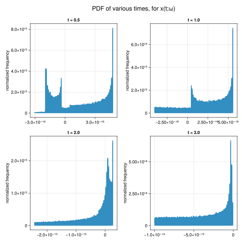
Compute the PDF of Equation 8 at times \(\{0.5, 1, 2, 3\}\) (use relative frequencies).

Note: you can debug your gPC results by either computing the analytic solution of Equation 7 and then computing moments/PDFs of such solutions as a function of \(t\), or by randomly sampling many solution paths of Equation 7 and then computing ensemble averages.

Solution

We have everything we need to compute the PDF of Equation 8 for various times.

Let us generate a random vector by sampling \(p_{\xi}(x)\) 50,000 times, then generate samples by evaluating the following:

\[\begin{align} x(t^*;\omega) = \sum_{i=0}^{6}\hat{x}_i(t^*) P_i(\xi(\omega)) \end{align}\]

where

\[\begin{align} &\hat{x}_i(t^*) &\quad &\text{are the gPC coefficients at time } t^* \\ &P_i(\xi) &\quad &\text{are the gPC basis functions} \\ &\xi &\quad &\text{random variables from the distribution } P_{\xi}(x) \end{align}\]

function question3b()
    # get orthogonal polynomials
    πn = stieltjes(μ, 6, sup)

    # get gPC modes
    sol = question3a()

    # generate samples of ξ
    r = LinRange(-1, 1, 1000)
    ys = hcat(cumsumtrap(μ, r), r)
    ξ_samples = Vector{Float64}(undef, 50000)
    for i in eachindex(ξ_samples)
        ξ_samples[i] = sampleInverseCDF(rand(), ys)
    end

    # define t*
    times = SVector{4}(0.5, 1.0, 2.0, 3.0)

    # number of solutions (gPC modes)
    M = size(sol)[1]

    # define figure
    fig = Figure(size = (800, 800))
    ax = SVector{4}(Axis(fig[1, 1]), Axis(fig[1, 2]), Axis(fig[2, 1]), Axis(fig[2, 2]))

    # plot histogram of samples of x(tstar;ω)
    for (i, tstar) in enumerate(times)
        hist!(ax[i], sum(sol(tstar)[j] .* πn[j].(ξ_samples) for j in 1:M), bins = 80, normalization = :pdf)
        ax[i].title = "t = $tstar"
        ax[i].ylabel = "normalized frequency"
    end
    Label(fig[0, :], "PDF of various times, for x(t;ω)", fontsize=20)
    save("question3b.png", fig)
end
question3b();

┌ Warning: No strict ticks found
└ @ PlotUtils ~/.julia/packages/PlotUtils/dVEMd/src/ticks.jl:194
┌ Warning: No strict ticks found
└ @ PlotUtils ~/.julia/packages/PlotUtils/dVEMd/src/ticks.jl:194

PDF for various times found by the method of relative frequencies

Appendix

Validation

Let us randomly sample many solution paths of Equation 7 and then compute the ensemble average to validate our gPC results.

For this we will generate 50,000 samples from the PDF of Equation 1, then solve the ODE numerically 50,000 times and plot the histogram of the normalized frequency just as we did in Question 3 partb.

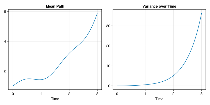
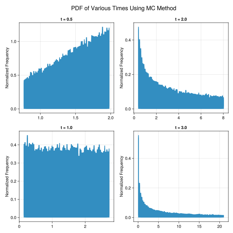
function validation(N::Int64)
    # generate samples of ξ
    r = LinRange(-1, 1, 1000)
    ys = hcat(cumsumtrap(μ, r), r)
    ξ_samples = Vector{Float64}(undef, N)
    for i in eachindex(ξ_samples)
        ξ_samples[i] = sampleInverseCDF(rand(), ys)
    end

    # define t*
    times = SVector{4}(0.5, 1.0, 2.0, 3.0)

    # define the ODEProblem
    function ode(u, p, t)
        return SVector{1}(-p * u[1] + cos(4*t))
    end

    # initial condition
    u0 = SVector{1}(1)

    # solve once to get size of time vector
    prob = ODEProblem(ode, u0, (0.0, 3.0), -1.0)
    sol = solve(prob, Tsit5(), saveat=0.01, abstol=1e-8, reltol=1e-8)

    # init matrix to store solutions
    solTstar = [Float64[] for _ in 1:length(times)]
    solutions = Matrix{Float64}(undef, N, size(sol.t)[1])

    # solve the ode for each sample and extract sample paths
    for (i, ξ) in enumerate(ξ_samples)
        prob = ODEProblem(ode, u0, (0.0, 3.0), ξ)
        sol = solve(prob, Tsit5(), saveat=0.01, abstol=1e-8, reltol=1e-8)
        solutions[i, :] = Float64[u[1] for u in sol.u]
        for (j, tstar) in enumerate(times)
            push!(solTstar[j], sol(tstar)[1])
        end
    end

    # calculate sample path mean and variance
    meanPath = mean(solutions, dims=1)
    variancePath = var(solutions, mean=meanPath, dims=1)

    # plot results
    fig1 = Figure(size = (800, 800))
    ax1 = [Axis(fig1[i, j]) for i in 1:2, j in 1:2]
    fig2 = Figure(size = (800, 400))
    ax2 = [Axis(fig2[1, i]) for i in 1:2]
    for (i, tstar) in enumerate(times)
        hist!(ax1[i], solTstar[i], bins = 80, normalization = :pdf)
        ax1[i].title = "t = $tstar"
        ax1[i].ylabel = "Normalized Frequency"
    end
    Label(fig1[0, :], "PDF of Various Times Using MC Method", fontsize=20)
    lines!(ax2[1], sol.t, vec(meanPath), label="Mean Path")
    ax2[1].title = "Mean Path"
    ax2[1].xlabel = "Time"
    lines!(ax2[2], sol.t, vec(variancePath), label="Variance")
    ax2[2].title = "Variance over Time"
    ax2[2].xlabel = "Time"
    save("validationPDF.png", fig1)
    save("validationmeanvar.png", fig2)
end
validation(50000);

The mean and variance of \(x(t;\omega)\) using Monte Carlo method

The PDF for specific times using Monte Carlo method

Footnotes

1. Note that \(\mathbb{E}\{\eta(\xi(\omega))P_k(\xi(\omega))\}\) can be computed with MC, or with quadrature as \[\mathbb{E}\{\eta(\xi(\omega))P_k(\xi(\omega))\}= \int_{-1}^{1}\frac{x - 1}{2 + 1 \sin(2x)}P_k(x)P_\xi(x)dx \tag{4}\]